Jupyter Notebook Tutorial
%matplotlib inline
import pylab as pl
import healpy as hp
import numpy as np
import h5py as h5
from PS4Cast  import *
import astropy
from astropy import units as u,  constants as C
dir_ps='path/to/PS4C/'
lens=np.array(hp.read_cl(dir_ps+'data/lensedCls.fits'))
l=(np.arange(len(lens[-1])))
tens=np.array(hp.read_cl(dir_ps+'data/r_0.05_tensCls.fits'))
cltot=[i+k  for i,k in zip(lens,tens)]
cbb_80=cltot[2][80]
cbb_1000=cltot[2][1000]
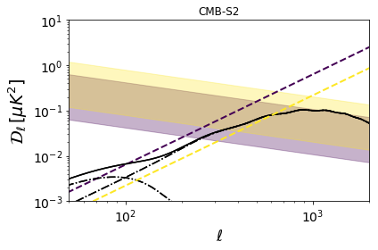
Current Ground Based
nu=[95,150]
sens=[0.1,0.1]
fwhm=[4,3.5]
fsky=.05

s2= Experiment(ID='CMB-S2', sensitivity= sens, frequency=nu , fwhm=fwhm , fsky=fsky,nchannels=2,
                units_sensitivity='Jy',units_beam='arcmin')
forecasts2=Forecaster(pb,  ps4c_dir=dir_ps, sigmadetection=3. )
forecasts2.forecast_pi2scaling(verbose=False)
forecasts2()
forecast2.plot_powerspectra(spectra_to_plot='Bonly',FG='total', xlim=[50,2000], ylim=[1e-3,1e1], savefig='../pspaper/cmbs2_Bmodes.pdf')
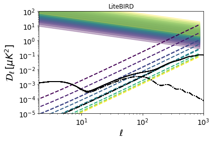
LiteBIRD
freqs=[40,50,60, 68, 78,89, 100,119, 140,166]
netarr=[53.4,32.3,25.1,19.6,15.3,12.4,15.6,12.6,8.3,8.7]
fwhms= [(C.c.cgs/(f*1e9/  u.s ) /(50.*u.cm)* u.rad ) .to(u.arcmin).value  for f in freqs]
fsky=.73
litebird= Experiment(ID='LiteBIRD', sensitivity=netarr, frequency=freqs ,nchannels=len(freqs), fwhm=fwhms , fsky=fsky,
                units_sensitivity='uKarcmin',units_beam='arcmin')
forecastlitebird=Forecaster(litebird,sigmadetection=3., ps4c_dir=dir_ps)
forecastlitebird.forecast_pi2scaling(verbose=False)

forecastlitebird(model='c2ex')
forecastlitebird.print_info()
=========================================================================================
LiteBIRD    Specifics

Frequency   ...... [  40.   50.   60.   68.   78.   89.  100.  119.  140.  166.] GHz
Flux limit  ...... [ 0.14589884  0.08824967  0.06857792  0.10710177  0.08360495  0.06775826
  0.08524426  0.06885114  0.09070864  0.09508014] Jy
Resolution  ...... [ 51.53052772  41.22442218  34.35368515  30.31207513  26.42591165
  23.15978774  20.61221109  17.32118579  14.72300792  12.41699463] arcmin
# channels  ...... 10
Fraction of sky     ...... 0.73
Beam angle  ...... [  2.54592634e-04   1.62939286e-04   1.13152282e-04   8.80943371e-05
   6.69540130e-05   5.14263622e-05   4.07348215e-05   2.87654978e-05
   2.07830722e-05   1.47825597e-05] sr
//////////////////////////////////////////////////////////////////////////////////////////
Forecasted quantities

Frequency   #sources[S,P]    Confusion       <Pi>    <Pi^2>x1e3     D^TT(lensing)   D^BB(lensing)

40.0 GHz    496     3       171.958mJy      4.26    2.17     15208.7 uK2      16.4795 uK2
50.0 GHz    913     9       98.5265mJy      4.28    2.25     3988.99 uK2      4.48189 uK2
60.0 GHz    957     6       46.2629mJy      4.30    2.33     1249.09 uK2      1.45431 uK2
68.0 GHz    571     3       33.8506mJy      4.31    2.39     1233.54 uK2      1.47706 uK2
78.0 GHz    763     4       24.0354mJy      4.33    2.48     602.159 uK2      0.746345 uK2
89.0 GHz    882     8       15.3532mJy      4.35    2.57     287.989 uK2      0.370506 uK2
100.0 GHz   679     7       11.4785mJy      4.37    2.67     250.716 uK2      0.334577 uK2
119.0 GHz   866     10      7.43595mJy      4.41    2.84     124.197 uK2      0.176284 uK2
140.0 GHz   488     4       2.05056mJy      4.45    3.03     84.9906 uK2      0.128869 uK2
166.0 GHz   462     4       1.47748mJy      4.50    3.28     65.0669 uK2      0.106753 uK2
==========================================================================================
forecastlitebird.plot_powerspectra(spectra_to_plot='Bonly', FG='total',
                                   savefig='litebird_Bmodes.pdf', xlim=[2,1000],ylim=[1e-5,1e2])