interfaces package

Submodules

interfaces.deflationlib module

interfaces.deflationlib.arnoldi(A, b, x0=None, tol=1e-05, maxiter=1000, inner_m=30)

Computes an orthonormal basis to get the approximated eigenvalues (Ritz eigenvalues) and eigenvector.

The basis comes from a Gram-Schmidt orthonormalization of the Krylov subspace defined as:

at the -th iteration.

Parameters

• A : {sparse matrix , linear operator}

  matrix we want to approximate eigenvectors;

• b : {array}

  array to build the Krylov subspace ;

• x0 : {array}

  initial guess vector to compute residuals;

• tol : {float}

  tolerance threshold to the Ritz eigenvalue computation;

• maxiter : {int}

  to validate the result one can compute maxiter times the eigenvalues, to seek the stability of the algorithm;

• inner_m : {int}

  maximum number of iterations within the Arnoldi algorithm,

  Warning

  inner_m <=N_pix

Returns

• w : {list of arrays}

  the orthonormal basis m x N_pix;

• h : {list of arrays}

  the elements of the Hessenberg matrix. At the m-th iteration has got elements.

interfaces.deflationlib.build_Z(z, y, w, eps)

Build the deflation matrix . Its columns are the selected eigenvectors s.t. their eigenvalues are smaller than a certain threshold eps.

Parameters

• z : {array}

  eigenvalues of ;

• y : {list of arrays}

  eigenvectors of ;

• w : {list of arrays}

  orthonormal basis (computed with the Arnoldi algorithm);

• eps : {float}

  threshold to select the smallest eigenvalues.

Returns

• Z : {matrix}

  deflation subspace matrix;

• r : {int}

  .

interfaces.deflationlib.build_hess(h, m)

Compute and store (as a Hessenberg matrix) the matrix from the output list h of the arnoldi() routine.

Parameters

• h : {list of arrays}

  matrix coefficients ;

• m : {int}

  size of H

Returns

• H :{numpy.matrix}

interfaces.deflationlib.find_ritz_eigenvalues(h, v, threshold=0.01)

interfaces.deflationlib.run_krypy_arnoldi(A, x0, M, tol, maxiter=None)

interfaces.linearoperators module

class interfaces.linearoperators.BlockDiagonalLO(CES, n, pol=1)

Bases: linop.linop.LinearOperator

Explicit implementation of , in order to save time in the application of the two matrices onto a vector (in this way the leading dimension will be instead of ).

Note

it is initialized as the BlockDiagonalPreconditionerLO since it involves computation with the same matrices.

mult(x)

Multiplication of on to a vector math:x ( array).

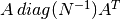
class interfaces.linearoperators.BlockDiagonalPreconditionerLO(CES, n, pol=1)

Bases: linop.linop.LinearOperator

Standard preconditioner defined as:

where is the pointing matrix (see SparseLO). Such inverse operator could be easily computed given the structure of the matrix . It could be sparse in the case of Intensity only analysis (pol=1), block-sparse if polarization is included (pol=3,2).

Parameters

• n:{int}

  the size of the problem, npix;

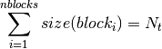
• CES:{ProcessTimeSamples}

  the linear operator related to the data sample processing. Its members (counts, masks, sine, cosine, etc... ) are needed to explicitly compute the inverse of the blocks of .

• pol:{int}

  the size of each block of the matrix.

mult(x)

Action of , where is an array.

class interfaces.linearoperators.BlockLO(blocksize, t, offdiag=False)

Bases: interfaces.blkop.BlockDiagonalLinearOperator

Derived class from blkop.BlockDiagonalLinearOperator. It basically relies on the definition of a block diagonal operator, composed by nblocks diagonal operators. If it does not have any off-diagonal terms (default case ), each block is a multiple of the identity characterized by the values listed in t and therefore is initialized by the BlockLO.build_blocks() as a linop.DiagonalOperator.

Parameters

• blocksize : {int or list }

  size of each diagonal block, if int it is : .

• t : {array}

  noise values for each block

• offdiag : {bool, default False}

  strictly related to the way the array t is passed (see notes ).

  Note

  • True : t is a list of array,

    shape(t)= [nblocks,bandsize], to have a Toeplitz band diagonal operator,

  • False : t is an array, shape(t)=[nblocks].

    each block is identified by a scalar value in the diagonal.

build_blocks()

Build each block of the operator either with or without off diagonal terms. Each block is initialized as a Toeplitz (either band or diagonal) linear operator.

self.diag: {numpy array}

the array resuming the .

build_unbalanced_blocks()

Build the list of Diagonal blocks of blk.BlockDiagonalLinearOperator by assuming that the blocks have different size. Of course it is required that:

isoffdiag

Property saying whether or not the operator has off-diagonal terms.

class interfaces.linearoperators.CoarseLO(Z, Az, r, apply='LU')

Bases: linop.linop.LinearOperator

This class contains all the operation involving the coarse operator . In this implementation is always applied to a vector wiht its inverse : . When initialized it performs either an LU or an eigenvalue decomposition to accelerate the performances of the inversion.

Parameters

• Z : {np.matrix}

  deflation matrix;

• A : {SparseLO}

  to compute vectors ;

• r : {int}

  , dimension of the deflation subspace;

• apply:{str}

  • LU: performs LU decomposition,
  • eig: compute the eigenvalues and eigenvectors of E.

mult(v)

Perform the multiplication of the inverse coarse operator . It exploits the LU decomposition of to solve the system . It first solves and then .

mult_eig(v)

Matrix vector multiplication with computed via setting_inverse_w_eigenvalues().

setting_inverse_w_eigenvalues(E)

This routine computes the inverse of E by a decomposition through an eigenvalue decomposition. It further checks whether it has some degenerate eigenvalues, i.e. 0 to numerical precision (1.e-15), and eventually excludes these eigenvalues from the anaysis.

class interfaces.linearoperators.DeflationLO(z)

Bases: linop.linop.LinearOperator

This class builds the Deflation operator (and its transpose) from the columns of the matrix Z.

Parameters

• z : {np.matrix}

  the deflation matrix. Its columns are read as arrays in a list self.z.

mult(x)

Performs the matrix vector multiplication with .

rmult(x)

Performs the product onto a N_pix vector with .

class interfaces.linearoperators.FilterLO(size, subscan_nsample, samples_per_bolopair, bolos_per_ces, pix_samples, poly_order=0)

Bases: linop.linop.LinearOperator

When applied to vector, this operator filters out Legendre Polynomial components from it up to a certain order. In the simple case of a order polynomial the effect

of filter consists of subtracting the offset from the samples.

Parameters

• size: {int}

  the size of the input array;

• subscan_nsample: {list of 2 array}

  • subscan_nsample[0], contains the size of each chunk of the samples

    which has to be processed;

  • subscan_nsample[1], contains the starting sample index of each chunk;

• samples_per_bolopair:{list of int }

  Number of samples observed during one Constant Elevation Scan (CES) for any pair of detectors. If more CES are included it is a list of int;

• bolos_per_ces:{list of int}

  Number of pairs of detectors that observed during a CES.

• pix_samples: {array}

  the same argument as in SparseLO, encoding all the pixels observed during observations.

• poly_order: {int}

  maximum order of polynomials to be subtracted from the samples.

Note

To be consistent with tha analysis FilterLO does not take into account all the flagged samples.

compute_legendres()

mult(d)

polyfilter(d)

polyfilter_multithreads(d)

procsfilter(args)

class interfaces.linearoperators.GroundFilterLO(ground)

Bases: linop.linop.LinearOperator

counts_in_groundbins(g)

mult(v)

class interfaces.linearoperators.InverseLO(A, method=None, preconditioner=None)

Bases: linop.linop.LinearOperator

Construct the inverse operator of a matrix , as a linear operator.

Parameters

• A : {linear operator}

  the linear operator of the linear system to invert;

• method : {function }

  the method to compute A^-1 (see below);

• P : {linear operator } (optional)

  the preconditioner for the computation of the inverse operator.

converged

provides convergence information:

• 0 : successful exit;
• >0 : convergence to tolerance not achieved, number of iterations;
• <0 : illegal input or breakdown.

isconverged(info)

It returns a Boolean value depending on the exit status of the solver.

Parameters

• info : {int}

  output of the solver method (usually scipy.sparse.cg()).

method

The method to compute the inverse of A. It can be any scipy.sparse.linalg solver, namely scipy.sparse.linalg.cg(), scipy.sparse.linalg.bicg(), etc.

mult(x)

It returns by solving the linear system with a certain scipy routine (e.g. scipy.sparse.linalg.cg()) defined above as method.

preconditioner

Preconditioner for the solver.

class interfaces.linearoperators.SparseLO(n, m, pix_samples, pol=1, angle_processed=None)

Bases: linop.linop.LinearOperator

Derived class from the one from the LinearOperator in linop. It constitutes an interface for dealing with the projection operator (pointing matrix).

Since this can be represented as a sparse matrix, it is initialized by an array of observed pixels which resembles the (i,j) positions of the non-null elements of the matrix,``obs_pixs``.

Parameters

• n : {int}

  size of the pixel domain ;

• m : {int}

  size of time domain; (or the non-null elements in a row of );

• pix_samples : {array}

  list of pixels observed in the time domain, (or the non-null elements in a row of );

• pol : {int,[default pol=1]}

  process an intensity only (pol=1), polarization only pol=2 and intensity+polarization map (pol=3);

• angle_processed: {ProcessTimeSamples}

  the class (instantiated befor SparseLO)has already computed the and , we link the cos and sin attributes of this class to the ProcessTimeSamples ones ;

maptype

Return a string depending on the map you are processing

mult(v)

Performs the product of a sparse matrix , with a numpy array () .

It extracts the components of corresponding to the non-null elements of the operator.

mult_iqu(v)

Performs the product of a sparse matrix , with v a numpy array containing the three Stokes parameters [IQU] .

Note

Compared to the operation mult this routine returns a -size vector defined as:

with is the pixel observed at time with polarization angle .

mult_qu(v)

Performs with being a polarization vector. The output array will encode a linear combination of the two Stokes parameters, (whose components are stored contiguously).

rmult(v)

Performs the product for the transpose operator .

rmult_iqu(v)

Performs the product for the transpose operator to get a IQU map-like vector. Since this vector resembles the pixel of 3 maps it has 3 times the size Npix. IQU values referring to the same pixel are contiguously stored in the memory.

rmult_qu(v)

Performs . The output vector will be a QU-map-like array.

class interfaces.linearoperators.ToeplitzLO(a, size)

Bases: linop.linop.LinearOperator

Derived Class from a LinearOperator. It exploit the symmetries of an dim x dim Toeplitz matrix. This particular kind of matrices satisfy the following relation:

Therefore, it is enough to initialize A by mean of an array a of size = dim.

Parameters

• a : {array, list}

  the array which resembles all the elements of the Toeplitz matrix;

• size : {int}

  size of the block.

mult(v)

Performs the product of a Toeplitz matrix with a vector x.

Module contents

This module contains the 2 main libraries for COSMOMAP2